INTRODUCTION:

The two criteria used for selecting a data structure and algorithm are the amount of memory required and the speed of execution. The analysis of the speed of an algorithm leads to a summary statement called the order of an algorithm.

The key topics for this lesson are:

A. Order of Algorithms
B. Constant Algorithms, O(1)
C. Log2N Algorithms, O(log2N)
D. Linear Algorithms, O(N)
E. N * Log2N Algorithms, O(N * log2N)
F. Quadratic Algorithms, (N2)
G. Other Orders
H. Comparison of Orders of Algorithms

VOCABULARY:

ORDER OF ALGORITHM
LOG2 N
N LOG2 N
CUBIC

CONSTANT
LINEAR
QUADRATIC
BIG O NOTATION

DISCUSSION:

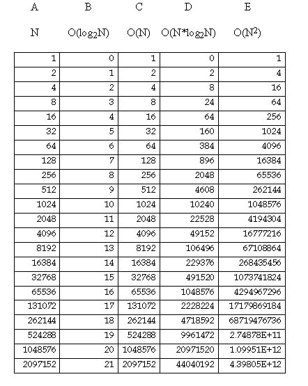
A. Order of Algorithms

1. The order of an algorithm is based on the number of steps that it takes to complete a task. Time is not a valid measuring stick because computers have different processing speeds. We want a method of comparing algorithms that is independent of computing environment and microprocessor speeds.

2. Most algorithms solve problems involving an amount of data, N. The order of algorithms will be expressed as a function of N, the size of the data set.

3. The following chart summarizes the numerical relationships of common functions of N.

a. The first column, N, is the number of items in a data set.
b. The other four columns are mathematical functions based on the size of N. In computer science, we write this with a capital O (order) instead of the traditional F (function) of mathematics. This type of notation is the order of an algorithm, or Big O notation.
c. You have already seen the last column in an empirical sense when you counted the number of steps in the quadratic sorting algorithms. The relationship between columns A and E is quadratic - as the value of N increases, the other column increases as a function of N2.

d. As we work through the rest of the student outline, assume the following array declaration of list applies:

int[] list = new int[4001];

Here are the specifications of array list:

1. Index position 0 keeps track of how many integers are stored as data.
2. Integers are stored from positions list[1] ... list[list[0]].

B. Constant Algorithms, O(1)

1. This relationship was not included in the chart. Here, the size of the data set does not affect the number of steps this type of algorithm takes. For example:\

int howBig (int[] list)
{
    return list[0];
}

2. The number of data in the array could vary from 0..4000, but this does not affect the algorithm of howBig. It will take one step regardless of how big the data set is.

3. A constant time algorithm could have more than just one step, as long as the number of steps is independent of the size (N) of the data set.

C. Log2N Algorithms, O(log2N)

1. A logarithm is the exponent to which a base number must be raised to equal a given number.

2. A log2N algorithm is one where the number of steps increases as a function of log2N. If the number of data was 1024, the number of steps equals log2 1024, or 10 steps.

3. Algorithms in this category involve splitting the data set in half repeatedly. Several examples will be encountered later in the course.

4. Algorithms which fit in this category are classed as O(log N), regardless of the numerical base used in the analysis.

D. Linear Algorithms, O(N)

1. This is an algorithm where the number of steps is directly proportional to the size of the data set. As N increases, the number of steps also increases.

long sumData (int[] list)
//  sums all the values in the array
{
  long total = 0;

  for (int loop = 1; loop <= list[0]; loop++)
  {
    total += list[loop];
  }
  return total;
}

2. In the above example, as the size of the array increases, so does the number of steps in the function.

3. A non-recursive linear algorithm, O(N), always has a loop involved.

4. Recursive algorithms are usually linear where the looping concept is developed through recursive calls. The recursive factorial function is a linear function.

long fact (int  n)
//  precondition:  n > 0
{
  if (1 == n)
    return 1;
  else
    return  n * fact(n - 1);
}

The number of calls of fact will be n. Inside of the function is one basic step, an if/then/else. So we are executing one statement n times.

E. N * Log2N Algorithms, O(N * log2N)

1. Algorithms of this type have a log N concept that must be applied N times.

2. When recursive MergeSort and Quicksort are covered, we will discover that they are O(N * log2N) algorithms.

3. These algorithms are markedly more efficient than our next category, quadratics.

F. Quadratic Algorithms, (N^2)

1. This is an algorithm where the number of steps required to solve a problem increases as a function of N2. For example, here is bubbleSort.

void bubbleSort (int[][] list)
{
  for (int outer = 1; outer <= list[0]-1; outer++)
  {
    for (int inner = 1; inner <= list[0]-outer; inner++)
    {
      if (list[inner] > list[inner + 1])
      {
        // swap list[inner] & list[inner + 1]
        int temp = list[inner];
        list[inner] = list[inner + 1]);
        list[inner + 1] = temp;
      }
    }
  }
}

2. The if statement is buried inside nested loops, each of which is tied to the size of the data set, N. The if statement is going to happen approximately N2 times.

3. The efficiency of this bubble sort was slightly improved by having the inner loop decrease. But we still categorize this as a quadratic algorithm.

4. For example, the number of times the inner loop happens varies from 1 to (N-1). On average, the inner loop occurs (N/2) times.

5. The outer loop happens (N-1) times, or rounded off N times.

6. The number of times the if statement is executed is equal to this expression:

# if statements = (Outer loop) * (Inner loop)
# if statements = (N) * (N/2)
# if statements = (N^2)/2

7. Ignoring the coefficient of 1/2, we have an algorithm that is quadratic in nature.

8. When determining the order of an algorithm, we are only concerned with its category, not a detailed analysis of the number of steps.

G. Other Orders

1. A cubic algorithm is one where the number of steps increases as a cube of N, or N^3.

2. An exponential algorithm is one where the number of steps increases as the power of a base, like 2^N.

3. Both of these categories are astronomical in the number of steps required. Such algorithms cannot be implemented on small personal computers.

H. Comparison of Orders of Algorithms

1. We obviously want to use the most efficient algorithm in our programs. Whenever possible, choose an algorithm that requires the fewest number of steps to process data.

2. The transparency, T.A.22.1, Order vs. Efficiency in Algorithms, summarizes all the categories in this lesson. Note that both axes in this diagram are exponential in scale.

SUMMARY/ REVIEW:

When designing solutions to programming problems, we are concerned with the most efficient solutions regarding time and space. We will consider memory requirements at a later time. Speed issues are resolved based on the number of steps required by algorithms.